2. Characteristics and equivalent model

2.1 Constant model

- Expression of the e.m.f

The armature being in rotation, the conductors cut the inductor magnetic flux and carry an alternating induced voltage. The collector rectifies this voltage; the number of slots being large, the e.m.f. between the brushes is almost continuous.

It is given by:

E = N.n.Ф       or        E = K.Ф.Ω

with: K = N/2π

E : e.m.f (V) ; N : number of active armature conductors ; Ф : flux under inductor pole (Wb) ; n and Ω : rotor speed (n in rev/s, and Ω in rad/s).

It can be noted that:

- The collector is a rotating voltage rectifier.

- If the flux is constant (most common case), E is directly proportional to the speed Ω.

- The current in the armature causes a magnetic field which modifies the e.m.f. This is the armature magnetic reaction, which is attenuated by arranging additional windings on the rotor. This phenomenon is generally neglected.

- Armature model

The armature model is given in Figure 13. It is governed by the equation:

U = E - R.I

E: e.m.f (V) ; U: armature voltage (V) ; I: armature current (A) ; R: armature resistance (Ω) which takes into account the winding, the collector and the brushes.

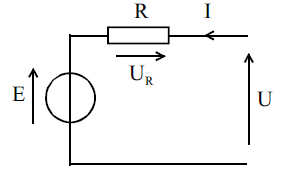
Figure 13: Armature model

 

- Moment of the electromagnetic torque

Electromagnetic power is converted into mechanical power.

P_em = E.I = T_em.Ω

With:  E = K.Ф.Ω. In this case, we find:

T_em = K.Ф.I

T_em: moment of the electromagnetic torque (N.m) ; Ф: flux under pole inductor (Wb) ; I: armature current (A).

 

- Expression of the speed

Using the Ohm's law and the expression for the e.m.f. give:

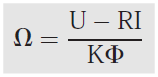
Ω: armature rotation speed (rad/s) ; U: armature voltage (V) ; I: armature current (A) ; R: armature resistance (Ω) ; Ф: flux under pole inductor (Wb).

 

- No-load characteristic

It is given for a generator with separate excitation, whatever the excitation mode of the machine. This is the magnetization curve of the magnetic circuit. The operating point P is located around the saturation zone in Figure 14.

 

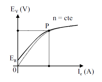
Figure 14: No-load characteristic

 

Due to hysteresis, the curve does not pass through the origin. There is a residual e.m.f. E_R (as well as a narrow hysteresis cycle, not shown in Figure 14).

 

2.2 Dynamic model

- Electrical and mechanical equations of the dynamic model

The equations of the dynamic model represented by Figure 15 are given by:

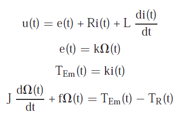
With: J: Moment of inertia; f: coefficient of viscous friction.

 

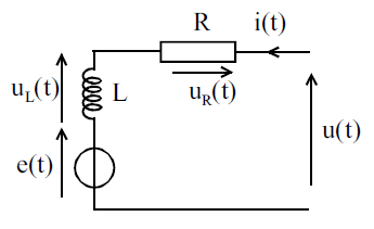
Figure 15: Equivalent armature diagram

 

- Block diagram of the dynamic model

The load and the supply voltage are the main cause of the speed variation, the motor is represented by a controlled system (Figure 16). Using Laplace's formulation, we have:

 

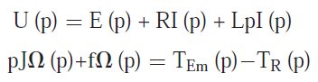
The block diagram of the dynamic model of the direct current machine is given in Figure 16.

 

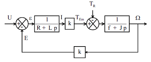
Figure 16 : Bloc diagram of the dynamic model

 

3. Separately excited motor

- Diagram

This excitation mode requires two separate power sources (Figure 17). The direction of rotation is changed by reversing the terminals of the armature or inductor.

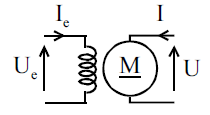
Figure 17: separately excited direct current machines

 

- Starting conditions

1. The inductor is supplied before the armature by adjusting the excitation current I_e to its rated value.

2. It is necessary to limit the armature current I_st at start-up (I_st < 2.I_N in general) by starting at reduced voltage, using a buck DC-DC converter or a controlled rectifier.

 

- Runaway condition

If the excitation is canceled while the armature is still supplied, the motor races and can destroy the armature. Consequently :

- We must never cut the excitation circuit.

- To stop the motor, we must cut the armature before the inductor (by reducing the armature voltage until the motor stops completely).

4. DC series motor (Series wound DC motor)

- Diagram

The inductor is in series with the armature: a single power source is sufficient. The direction of rotation is changed by reversing the connections of the armature and the inductor (figure 18).

The armature voltage becomes:

U = E + R_T.I

with: R_T = r + R

R : armature resistance (Ω) ; r : inductor résistance (Ω).

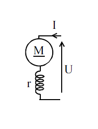
Figure 18: DC series motor

 

- Starting conditions and runaway conditions

1. The starting current must be limited as in separate excitation (I_D < 2.I_N in general).

2. We must never start without load under rated voltage, otherwise the motor will race and the armature may be destroyed.

 

5. Efficiency

- Power tree

Powers and losses of the direct current machine are given in figure 19.

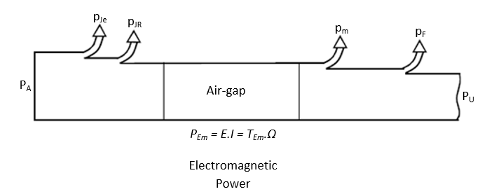
Figure 19: Power tree

The absorbed power is given by:

P_A = U.I + U_e.I_e

The copper losses in the armature are:

p_JR = R.I²

The copper losses in the inductor are:

p_Je = r.I_e² = U_e²/r = U_e.I_e

The useful power:

P_U = T_U.Ω

with: U: armature voltage (V) ; U_e: inductor voltage (V) ; I: armatre current ; I_e :inductor current (A) ; R: armature resistance (Ω) ; r : inductor resistance (Ω) ; T_U : useful torque on the shaft (N.m) ; Ω : rotor speed (rad/s).

 

It should be noted that:

- At constant speed, mechanical losses (p_m) and iron losses (p_F) are constant.

- The losses are grouped under the name of collective losses, i.e.: p_C = p_F + p_m, which, to a first approximation, are proportional to the speed.

 

- Efficiency

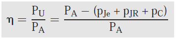
The motor efficiency is given by: