Chapter I: Introduction to Operations Research
Welcome to Operations Research!
Discover how mathematics and computational methods help solve real-world decision-making problems across industries, governments, and daily life.
1. What is Operations Research?
Definition
Operations Research (OR) is a scientific approach to decision-making that seeks to determine how best to design and operate systems, usually under conditions requiring the allocation of scarce resources.
"The set of rational methods and techniques oriented toward finding the best choice in how to operate in order to achieve the desired result or the best possible result."
Core Principles of OR
- Quantitative Analysis: Uses mathematical models and data to represent real situations
- Optimization: Seeks the best solution among many alternatives
- Scientific Methodology: Systematic, repeatable approach to problem-solving
- Decision Support: Provides insights and recommendations to decision-makers
- Systems Perspective: Considers interactions between different parts of a system
💡 Think About It:
When you plan your daily schedule, allocate your study time, or choose the fastest route to university; you're already doing informal operations research!
2. Historical Development of Operations Research
The Birth of OR: World War II (1939-1945)
The Challenge: British military needed to optimize radar placement to defend against German air attacks.
The Innovation: Physicist Patrick Blackett assembled a multidisciplinary team; the first "Operational Research" group, to apply scientific methods to military operations.
The Success: Mathematical analysis dramatically improved resource allocation, aircraft deployment, and defense strategies.
Key Insight: Complex operational problems could be solved using quantitative analysis, not just intuition.
Post-War Evolution: Timeline
| Era | Key Developments | Impact |
|---|---|---|
| 1947 | George Dantzig invents the Simplex Algorithm | Revolutionary method for solving linear programming problems |
| 1950s | Civilian applications begin (Air France, SNCF) | OR spreads to transportation, logistics, production |
| 1960s-70s | Development of computers | Ability to solve larger, more complex problems |
| 1980s-90s | Personal computers and software explosion | OR tools become accessible to all organizations |
| 2000s-Today | Big data, AI, machine learning integration | OR powers modern optimization in all sectors |
✅ Fun Fact:
The famous meeting between George Dantzig and mathematician John von Neumann on October 3, 1947, led to the development of duality theory, one of the most important concepts in optimization!
3. Modern Application Domains
🏭 Manufacturing & Production
- Production planning and scheduling
- Inventory management
- Quality control optimization
- Supply chain design
- Facility location and layout
Example: Toyota Production System uses OR principles
✈️ Transportation & Logistics
- Route optimization
- Vehicle routing and scheduling
- Crew assignment
- Warehouse management
- Network design
Example: UPS ORION system saves 100M+ miles annually
💰 Finance & Economics
- Portfolio optimization
- Risk management
- Asset allocation
- Trading strategies
- Credit scoring
Example: Modern portfolio theory by Harry Markowitz
🏥 Healthcare
- Hospital resource allocation
- Staff scheduling
- Treatment planning
- Emergency response
- Epidemic modeling
Example: Operating room scheduling optimization
🌍 Energy & Environment
- Power grid optimization
- Renewable energy planning
- Pollution control
- Resource management
- Climate modeling
Example: Smart grid energy distribution
💻 Technology & Telecom
- Network design and optimization
- Data center resource allocation
- Cloud computing optimization
- Algorithm efficiency
- Machine learning training
Example: Google's data center cooling optimization
4. Types of Problems in Operations Research
Classification by Nature
Type 1: Combinatorial Problems
Characteristic: Large (often enormous) number of possible solutions
Challenge: Finding the best solution among billions of possibilities
Example: Choosing 5 warehouse locations from 30 potential sites
- Number of combinations: C(30,5) = 142,506 possible selections!
- Must evaluate which combination minimizes total transportation cost
Solution Methods: Branch and bound, dynamic programming, heuristics
Type 2: Stochastic (Probabilistic) Problems
Characteristic: Involve uncertainty and randomness
Challenge: Must account for variability in data
Example: Inventory management with uncertain demand
- Customer demand varies randomly each day
- Must balance inventory costs vs. stockout risk
Solution Methods: Probability theory, simulation, stochastic programming
Type 3: Competitive Problems
Characteristic: Multiple decision-makers with conflicting objectives
Challenge: Each player's decision affects others
Example: Pricing strategies in competitive markets
- Two companies compete for same customers
- Each must anticipate competitor's actions
Solution Methods: Game theory, Nash equilibrium analysis
5. Introduction to Linear Programming (LP)
What is Linear Programming?
Linear Programming is a mathematical method for determining the optimal allocation of limited resources among competing activities, where both the objective and constraints are expressed as linear functions.
The Three Essential Components
1️⃣ Decision Variables
What they represent: The quantities we control and want to determine
Notation: x₁, x₂, ..., xₙ
Example:
- x₁ = units of Product A to produce
- x₂ = units of Product B to produce
2️⃣ Objective Function
What it represents: The goal we want to optimize (maximize or minimize)
Form: z = c₁x₁ + c₂x₂ + ... + cₙxₙ
Example:
- Maximize profit: z = 150x₁ + 100x₂
- Minimize cost: z = 5x₁ + 3x₂
3️⃣ Constraints
What they represent: Limitations and requirements
Form: Linear inequalities or equalities
Example:
- Material limit: 2x₁ + x₂ ≤ 400
- Non-negativity: x₁, x₂ ≥ 0
Four Fundamental Assumptions of Linear Programming
| Assumption | Meaning | Example/Implication |
|---|---|---|
| 1. Non-negativity | All decision variables must be ≥ 0 | Can't produce negative quantities or work negative hours |
| 2. Linearity | Objective function is a linear combination of variables | No x₁×x₂ terms, no x₁² terms; proportional relationships |
| 3. Constraint Linearity | All constraints are linear | Creates convex feasible region (important for optimization!) |
| 4. Certainty | All parameters are known constants | Distinguishes LP from stochastic programming |
6. Mathematical Formulation of LP Problems
Standard Form of a Linear Program
Optimize (Maximize or Minimize):
z = c₁x₁ + c₂x₂ + ... + cₙxₙ
Subject to:
a₁₁x₁ + a₁₂x₂ + ... + a₁ₙxₙ ≤ b₁
a₂₁x₁ + a₂₂x₂ + ... + a₂ₙxₙ ≤ b₂
...
aₘ₁x₁ + aₘ₂x₂ + ... + aₘₙxₙ ≤ bₘ
Non-negativity:
x₁, x₂, ..., xₙ ≥ 0
Matrix Notation (Compact Form)
Optimize: z = cᵀx
Subject to: Ax ≤ b, x ≥ 0
Where:
- x = (x₁, x₂, ..., xₙ)ᵀ is the decision variable vector (n × 1)
- c = (c₁, c₂, ..., cₙ)ᵀ is the objective coefficient vector (n × 1)
- A = [aᵢⱼ] is the constraint matrix (m × n)
- b = (b₁, b₂, ..., bₘ)ᵀ is the right-hand side vector (m × 1)
💡 Why Matrix Notation? Cleaner, more compact, easier for computer implementation, and essential for theoretical analysis!
7. How to Formulate an LP Problem: Step-by-Step
The Three-Step Modeling Process
Step 1: Identify Decision Variables
Ask yourself:
- What quantities can I control?
- What am I trying to determine?
- What decisions need to be made?
Tip: Use clear, descriptive notation (e.g., x₁ = "units of Product A", not just x₁)
Step 2: Formulate Constraints
Ask yourself:
- What limitations do I face?
- What resources are limited?
- Are there any minimum requirements?
- Are there any logical restrictions?
Tip: Always include non-negativity constraints at the end!
Step 3: Define Objective Function
Ask yourself:
- What is my goal?
- Do I want to maximize (profit, efficiency) or minimize (cost, time)?
- How does each variable contribute to my goal?
Tip: Make sure objective and constraints use the same units and time frame!
8. Complete Example: Production Planning Problem
Problem Statement
A furniture company produces two products: chairs (Product A) and tables (Product B).
Resource Requirements:
| Resource | Chair (A) | Table (B) | Available |
|---|---|---|---|
| Wood (kg) | 2 kg | 5 kg | 400 kg |
| Labor (hours) | 3 hours | 4 hours | 600 hours |
| Profit per unit | $50 | $80 | — |
🎯 Management Question: How many chairs and tables should the company produce to maximize total profit?
Solution: Step-by-Step Formulation
Step 1: Define Decision Variables
Let x₁ = number of chairs to produce
Let x₂ = number of tables to produce
Step 2: Formulate Objective Function
We want to maximize total profit:
Maximize: z = 50x₁ + 80x₂
(Each chair contributes $50, each table contributes $80)
Step 3: Write Constraints
Wood constraint:
2x₁ + 5x₂ ≤ 400
(Each chair uses 2 kg, each table uses 5 kg, total available: 400 kg)
Labor constraint:
3x₁ + 4x₂ ≤ 600
(Each chair needs 3 hours, each table needs 4 hours, total available: 600 hours)
Non-negativity:
x₁, x₂ ≥ 0
(Cannot produce negative quantities)
✅ Complete Formulation
Maximize: z = 50x₁ + 80x₂
Subject to:
2x₁ + 5x₂ ≤ 400 (Wood)
3x₁ + 4x₂ ≤ 600 (Labor)
x₁, x₂ ≥ 0 (Non-negativity)
9. The Graphical Solution Method (For 2-Variable Problems)
When Can We Use the Graphical Method?
- Only works for problems with two decision variables (x₁ and x₂)
- Provides excellent visual understanding of LP concepts
- Shows feasible region, constraints, and optimization graphically
- Great for learning, but impractical for larger problems
Step-by-Step Graphical Solution Process
Step 1: Set Up Coordinate System
- Horizontal axis (x-axis) represents x₁
- Vertical axis (y-axis) represents x₂
- Only plot the first quadrant (both variables ≥ 0)
Step 2: Plot Each Constraint
For each constraint:
- Convert inequality to equality (replace ≤ with =)
- Find two points on the line (usually intercepts)
- Draw the line
- Determine which side satisfies the inequality (shade feasible region)
Example for 2x₁ + x₂ ≤ 400:
- When x₁ = 0: x₂ = 400 → Point (0, 400)
- When x₂ = 0: x₁ = 200 → Point (200, 0)
- Draw line through these points
- Test point (0,0): 2(0) + (0) = 0 ≤ 400 ✓ → Shade toward origin
Step 3: Identify Feasible Region
- The feasible region is where ALL constraints are satisfied simultaneously
- It's the intersection (overlap) of all individual constraint regions
- For LP problems, this is always a convex polygon
Step 4: Find Corner Points (Vertices)
- The optimal solution is always at a corner point (vertex) of the feasible region
- Find coordinates of all corner points by solving systems of equations
- Include intersection points and axis intercepts
Step 5: Evaluate Objective Function
- Calculate the objective function value at each corner point
- The corner point with the best objective value is the optimal solution
🔑 Fundamental Theorem of Linear Programming
If an optimal solution exists, it occurs at a vertex (corner point) of the feasible region.
This is why we only need to check corner points—we don't need to test every point inside the region!
Complete Worked Example: Production Planning
Problem Statement
A company produces two products: Product A and Product B. The company uses three raw materials (M1, M2, M3) with limited availability.
Resource Requirements and Profit:
| Resource | Product A | Product B | Available |
|---|---|---|---|
| Material M1 (units) | 1 unit | 1 unit | 300 units |
| Material M2 (units) | 2 units | 1 unit | 400 units |
| Material M3 (units) | 0 units | 1 unit | 250 units |
| Profit per unit | $150 | $100 | — |
🎯 Question: How many units of Product A and Product B should the company produce to maximize total profit?
Mathematical Formulation
Step 1: Decision Variables
x₁ = units of Product A to produce
x₂ = units of Product B to produce
Step 2: Objective Function
We want to maximize total profit:
Maximize: z = 150x₁ + 100x₂
Step 3: Constraints
Material M1 constraint: x₁ + x₂ ≤ 300
Material M2 constraint: 2x₁ + x₂ ≤ 400
Material M3 constraint: x₂ ≤ 250
Non-negativity: x₁, x₂ ≥ 0
Graphical Solution Process
Step 1: Plot the Constraint Lines
Constraint 1: x₁ + x₂ = 300
- When x₁ = 0: x₂ = 300 → Point (0, 300)
- When x₂ = 0: x₁ = 300 → Point (300, 0)
- Feasible side: x₁ + x₂ ≤ 300 (toward origin)
Constraint 2: 2x₁ + x₂ = 400
- When x₁ = 0: x₂ = 400 → Point (0, 400)
- When x₂ = 0: x₁ = 200 → Point (200, 0)
- Feasible side: 2x₁ + x₂ ≤ 400 (toward origin)
Constraint 3: x₂ = 250
- Horizontal line at x₂ = 250
- Feasible side: x₂ ≤ 250 (below the line)
Step 2: Identify Corner Points
The feasible region is bounded by the constraints and the axes. We need to find all corner points:
Corner Point A: Origin
(0, 0) — Intersection of x₁ = 0 and x₂ = 0
Corner Point B: x₁-axis intercept
Intersection of x₂ = 0 and 2x₁ + x₂ = 400:
2x₁ + 0 = 400 → x₁ = 200
Point: (200, 0)
Corner Point C: Intersection of M1 and M2 constraints
Solve system:
x₁ + x₂ = 300
2x₁ + x₂ = 400
Subtract first from second:
x₁ = 100
x₂ = 300 - 100 = 200
Point: (100, 200)
Corner Point D: Intersection of M1 and M3 constraints
Solve system:
x₁ + x₂ = 300
x₂ = 250
Substitute:
x₁ + 250 = 300 → x₁ = 50
Point: (50, 250)
Corner Point E: Intersection of M3 and x₁-axis
(0, 250) — Intersection of x₁ = 0 and x₂ = 250
Step 3: Evaluate Objective Function at Each Corner Point
| Corner Point | Coordinates (x₁, x₂) | Objective Function z = 150x₁ + 100x₂ | Profit ($) |
|---|---|---|---|
| A | (0, 0) | 150(0) + 100(0) | $0 |
| B | (200, 0) | 150(200) + 100(0) | $30,000 |
| C | (100, 200) | 150(100) + 100(200) | $35,000 |
| D | (50, 250) | 150(50) + 100(250) | $32,500 |
| E | (0, 250) | 150(0) + 100(250) | $25,000 |
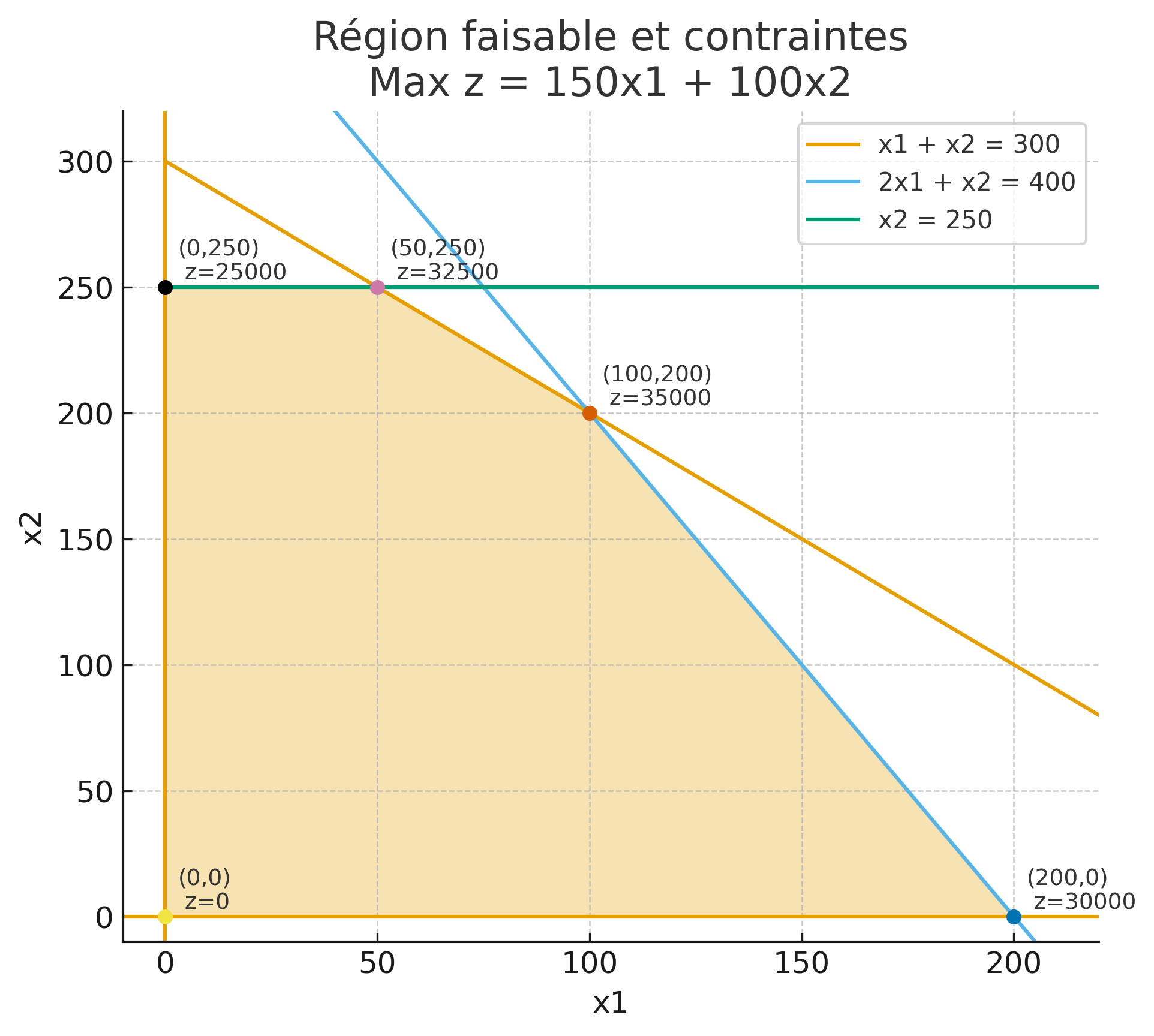
🎉 Optimal Solution
Optimal Production Plan:
• Produce 100 units of Product A
• Produce 200 units of Product B
Maximum Profit: $35,000
Resource Utilization:
- Material M1: 100 + 200 = 300 units (fully utilized ✓)
- Material M2: 2(100) + 200 = 400 units (fully utilized ✓)
- Material M3: 200 units used out of 250 available (50 units slack)
💡 Interpretation: Materials M1 and M2 are the binding constraints (fully used), while M3 has excess capacity. If we could obtain more M1 or M2, we could increase profit!
🔍 Key Insights from This Example
- Corner point optimality: The optimal solution occurred at vertex C, confirming the fundamental theorem
- Binding constraints: M1 and M2 are tight (no slack), meaning they limit production
- Non-binding constraint: M3 has 50 units of slack—not fully utilized
- Sensitivity: Additional units of M1 or M2 would increase profit (shadow prices > 0)
- Trade-offs: Product A has higher unit profit ($150 vs $100), but requires more M2
✅ Verification
Let's verify that our solution (100, 200) satisfies all constraints:
- M1: 100 + 200 = 300 ≤ 300 ✓
- M2: 2(100) + 200 = 400 ≤ 400 ✓
- M3: 200 ≤ 250 ✓
- Non-negativity: x₁ = 100 ≥ 0, x₂ = 200 ≥ 0 ✓
All constraints satisfied! ✓
10. The Simplex Algorithm: Solving Larger Problems
Why Do We Need the Simplex Algorithm?
- Graphical method only works for 2-variable problems
- Real-world problems often have hundreds or thousands of variables!
- Need systematic, computerizable method for large-scale problems
- Simplex algorithm: invented by George Dantzig in 1947
How the Simplex Algorithm Works
Geometric Intuition
Imagine you're standing at a corner of the feasible region (a multi-dimensional polyhedron):
- Look at all adjacent corners (neighbors connected by an edge)
- Move to an adjacent corner that improves the objective function
- Repeat until no adjacent corner offers improvement
- You've found the optimum!
💡 Key Insight: The algorithm intelligently "walks" along edges of the feasible region, always improving (or staying the same), never backtracking.
Simplex Algorithm Steps
Step 1: Initialization
Convert problem to standard form
Add slack variables to convert inequalities to equalities
Find an initial basic feasible solution (usually origin)
Step 2: Optimality Test
Check if current solution is optimal
Examine reduced costs (or relative cost coefficients)
If all ≤ 0 for maximization: STOP, optimal found!
Step 3: Select Entering Variable
Choose variable to enter the basis
Select variable with most positive reduced cost
This variable will increase from 0 to some positive value
Step 4: Unboundedness Test
Check if problem is unbounded
If entering variable can increase indefinitely: problem is unbounded
Otherwise, proceed to next step
Step 5: Select Leaving Variable
Determine which variable will leave the basis
Use minimum ratio test
Ensures feasibility is maintained
Step 6: Pivot Operation
Perform pivoting (row operations)
Update the simplex tableau
Move to new corner point
⚡ Efficiency of Simplex
Dantzig's Observation: "Most of the time, the simplex method solved problems in 2nd or 3rd steps, something impressive."
In practice, simplex usually finds the optimum in a number of iterations roughly equal to the number of constraints, far fewer than the total number of corner points!
📌 Important Notes
- Worst-case: Simplex can theoretically visit all corner points (exponential time)
- Average-case: Extremely efficient in practice (polynomial-like behavior)
- Alternatives: Interior point methods provide polynomial worst-case guarantees
- Software: Modern solvers use sophisticated variants of simplex
11. Duality Theory in Linear Programming
What is Duality?
Every linear programming problem has an associated "twin" problem called the dual. The original problem is called the primal.
Remarkable property: The dual of the dual is the primal! They are mathematical twins.
Primal-Dual Relationship
| Primal Element | ↔ | Dual Element |
|---|---|---|
| Maximize | ↔ | Minimize |
| n variables | ↔ | n constraints |
| m constraints | ↔ | m variables |
| Objective coefficients (c) | ↔ | Right-hand sides (b) |
| Right-hand sides (b) | ↔ | Objective coefficients |
| Constraint matrix A | ↔ | Transpose AT |
| ≤ constraints | ↔ | ≥ 0 variables |
Economic Interpretation of Duality
The Resource Valuation Perspective
Primal Problem: A manufacturer deciding production quantities to maximize profit
- Variables: How many units of each product to make
- Constraints: Limited resources (materials, labor, equipment)
- Objective: Maximize total profit
Dual Problem: A buyer offering to purchase the manufacturer's resources
- Variables: Price to offer for each unit of resource (shadow prices)
- Constraints: Total cost of resources must justify producing each product
- Objective: Minimize total payment for all resources
💰 Dual Variables = Shadow Prices
The optimal dual variable values tell you the marginal value of each resource, how much profit would increase if you had one more unit of that resource!
Fundamental Duality Theorems
Weak Duality Theorem
For any feasible solution x of the primal and any feasible solution y of the dual:
Primal Objective ≤ Dual Objective
Implication: The dual provides an upper bound on the primal optimal value (for maximization problems)
Strong Duality Theorem
If the primal has an optimal solution x*, then the dual also has an optimal solution y*, and:
Primal Optimal Value = Dual Optimal Value
Implication: The optimal values are equal! This is a profound mathematical result.
Complementary Slackness Theorem
At optimality, for each primal constraint and corresponding dual variable:
- If a primal constraint is not tight (has slack), the corresponding dual variable = 0
- If a dual variable is positive, the corresponding primal constraint must be tight
Interpretation: Resources with slack have zero shadow price; resources fully utilized have positive shadow price
Practical Applications of Duality
1. Bounds on Optimal Value
Use dual to quickly find upper/lower bounds without fully solving the primal
2. Sensitivity Analysis
Shadow prices show how objective changes with resource availability
3. Computational Efficiency
Sometimes the dual is easier to solve than the primal (fewer constraints or variables)
4. Economic Insights
Shadow prices reveal resource valuations for strategic decision-making
12. Real-World Impact and Success Stories
Industries Transformed by Operations Research
✈️ Aviation: American Airlines
Application: Crew scheduling, route optimization, fleet assignment
Impact: Saves over $500 million annually
Methods: Large-scale LP, integer programming, network optimization
📦 Logistics: UPS ORION System
Application: Route optimization for delivery drivers
Impact: Saves 100+ million miles per year, reduces fuel costs and emissions
Methods: Vehicle routing algorithms, real-time optimization
🏭 Manufacturing: Toyota Production System
Application: Just-in-time production, inventory minimization
Impact: Revolutionary lean manufacturing principles
Methods: Scheduling algorithms, inventory theory, quality control
💰 Finance: Portfolio Optimization
Application: Asset allocation, risk management
Impact: Foundation of modern investment theory (Nobel Prize: Markowitz, 1990)
Methods: Quadratic programming, stochastic optimization
13. Key Takeaways and Summary
What You've Learned
🎯 OR Fundamentals
- Scientific approach to decision-making
- Mathematical modeling of reality
- Optimization under constraints
📐 Linear Programming
- Three components: variables, objective, constraints
- Graphical method for 2-variable problems
- Simplex algorithm for larger problems
🔄 Duality Theory
- Every LP has a dual twin
- Shadow prices = resource values
- Powerful for sensitivity analysis
🌍 Real-World Impact
- Billion-dollar savings in industries
- Wide application across sectors
- Foundation for modern optimization
💡 Remember
Operations Research is not just about mathematics, it's about making better decisions. The models and algorithms are tools to help us understand complex systems and find optimal solutions to real-world problems.
14. Looking Ahead: Your OR Journey
Upcoming Chapters
- Chapter II: Integer & Boolean Programming, when variables must be whole numbers
- Chapter III: Scheduling (MPM, PERT), managing project timelines and resources
- Chapter IV: Convex Programming, extending beyond linear objectives
- Chapter V: Unconstrained Optimization, gradient methods and beyond
- Chapter VI: Real-World Applications, putting it all together with software
- Chapter VII: Advanced Topics, AI, emerging techniques, industry trends
15. Study Resources and Practice Tips
📚 How to Succeed in This Course
Active Learning Strategies:
- Practice formulation: Try to model everyday decisions as LP problems
- Work through examples: Don't just read, solve problems step by step
- Use graphical method: Visualize 2-variable problems to build intuition
- Check your work: Verify solutions make sense in the original context
- Discuss with peers: Explain concepts to others to deepen understanding
Recommended Practice:
- Solve at least 3-5 formulation problems
- Practice graphical method until it becomes automatic
- Review lecture slides and annotate with your own examples
💻 Software and Tools
You'll learn to use:
- Excel Solver: Quick LP solutions and sensitivity analysis
- Python (PuLP, scipy.optimize): Programming your own models
- AMPL/GAMS: Professional optimization modeling languages
- MATLAB: Numerical methods and algorithm implementation
Tip: Start with graphical/manual solutions to understand the concepts, then move to software for efficiency!
16. Chapter Activities and Self-Assessment
✅ Self-Check Questions
Test your understanding:
- Can you explain what operations research is in your own words?
- What are the three essential components of any linear programming problem?
- Why must all LP variables be non-negative?
- When can you use the graphical method to solve an LP problem?
- What is the geometric interpretation of the simplex algorithm?
- What does a "shadow price" tell you about a resource?
- Why is the optimal solution always at a corner point of the feasible region?
📝 Reflection Activity
Think about your own field of interest:
- Where might linear programming be applied in your future career?
- What kinds of resources need to be optimally allocated?
- What decisions could benefit from mathematical modeling?
Discuss your ideas with classmates or in the course forum!
17. Additional Resources and Further Reading
📖 Recommended Textbooks
- Introduction to Operations Research by Hillier & Lieberman (classic, comprehensive)
- Linear Programming by Vasek Chvátal (mathematical depth)
- Operations Research: Applications and Algorithms by Wayne Winston (practical focus)
🌐 Online Resources
- MIT OpenCourseWare: Free video lectures on optimization
- INFORMS (Institute for Operations Research): Professional resources and case studies
- YouTube: Search for "linear programming tutorial" for visual explanations
- Coursera/edX: Online courses on optimization and OR