Convex Programming

Part 1

Introduction to Convex Programming

• Convex sets & functions
• Partial derivatives & gradient
• Lagrange multipliers
• Optimality conditions

Part 2

Frank-Wolfe Method

• Conditional gradient algorithm
• Linear approximation approach
• Convergence analysis
• Practical applications

Part 3

Kelley's Cutting Plane Method

• Piecewise linear models
• Iterative refinement
• Bundle methods
• Non-differentiable functions

🎯 General Form

where \(f\) and \(g_i\) are convex functions, and \(h_j\) are affine functions (linear).

📘 Definition

A set \(C \subseteq \mathbb{R}^n\) is convex if for any two points \(x, y \in C\) and any \(\lambda \in [0,1]\):

In simple terms: The line segment connecting any two points in the set remains entirely within the set.

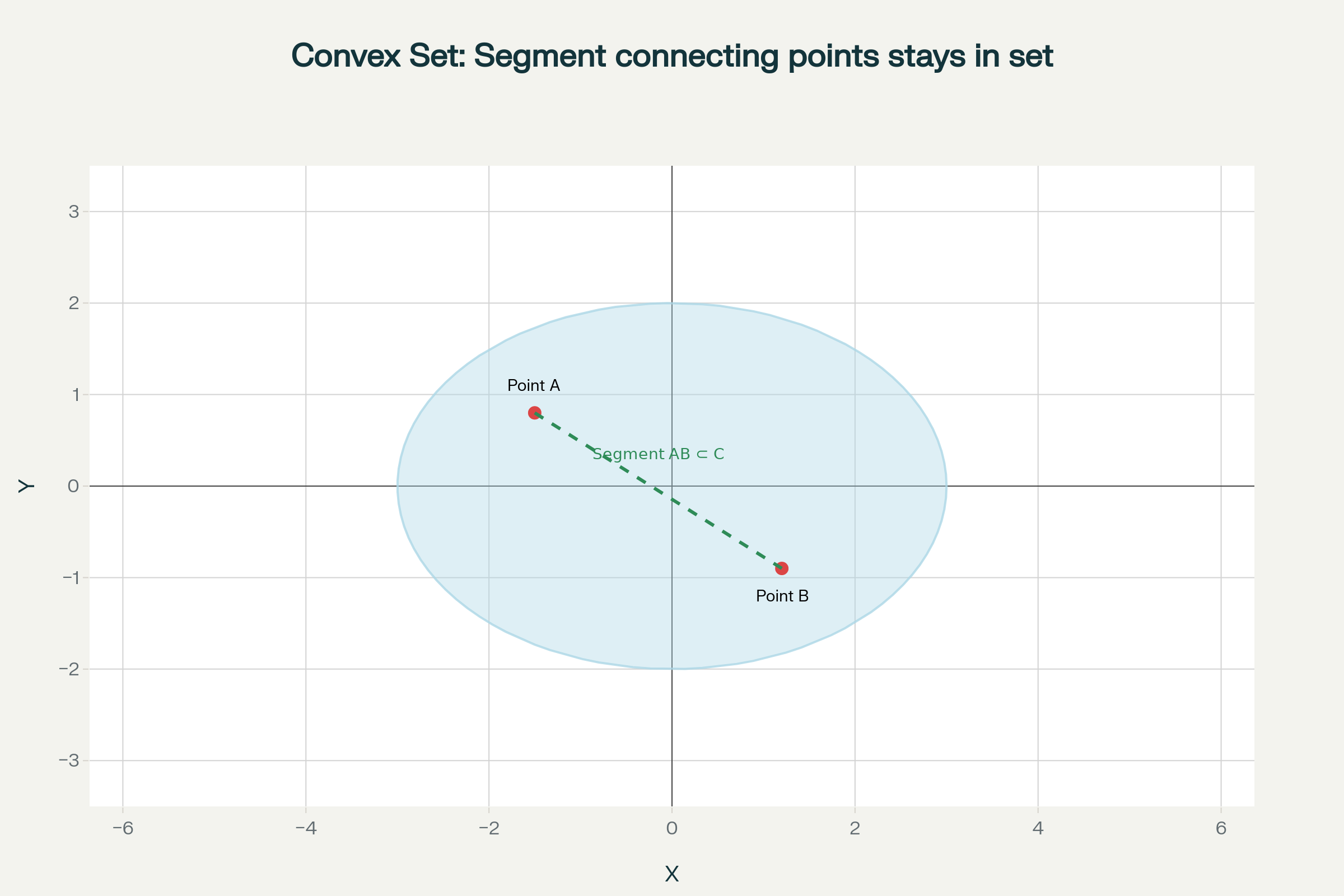
Figure 1: Illustration of a convex set. For all points A and B in C, the segment [AB] remains entirely in C.

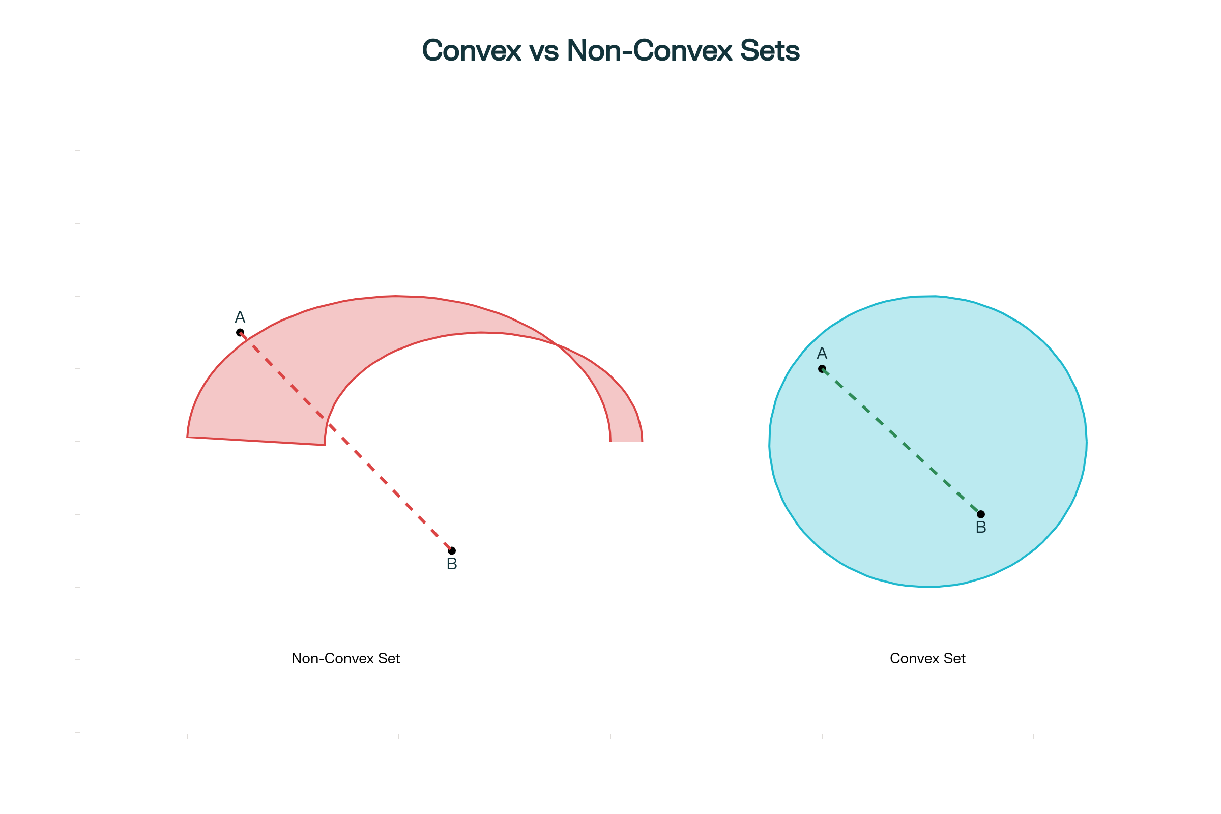
Figure 2: Comparison between convex and non-convex sets

💡 Examples of Convex Sets

• Empty set ∅ and singleton {x}: Trivially convex
• Euclidean space \(\mathbb{R}^n\): The entire space
• Halfspaces: \(\{x : a^Tx \leq b\}\)
• Polyhedra: Intersection of halfspaces
• Balls: \(\{x : \|x - x_c\| \leq r\}\)
• Ellipsoids: \(\{x : (x-x_c)^TP^{-1}(x-x_c) \leq 1\}\)

📘 Definition

A function \(f: \mathbb{R}^n \to \mathbb{R}\) is convex if its domain is convex and for any \(x, y\) in the domain and any \(\lambda \in [0,1]\):

Geometric interpretation: The chord connecting any two points on the graph of \(f\) always lies above (or on) the function curve.

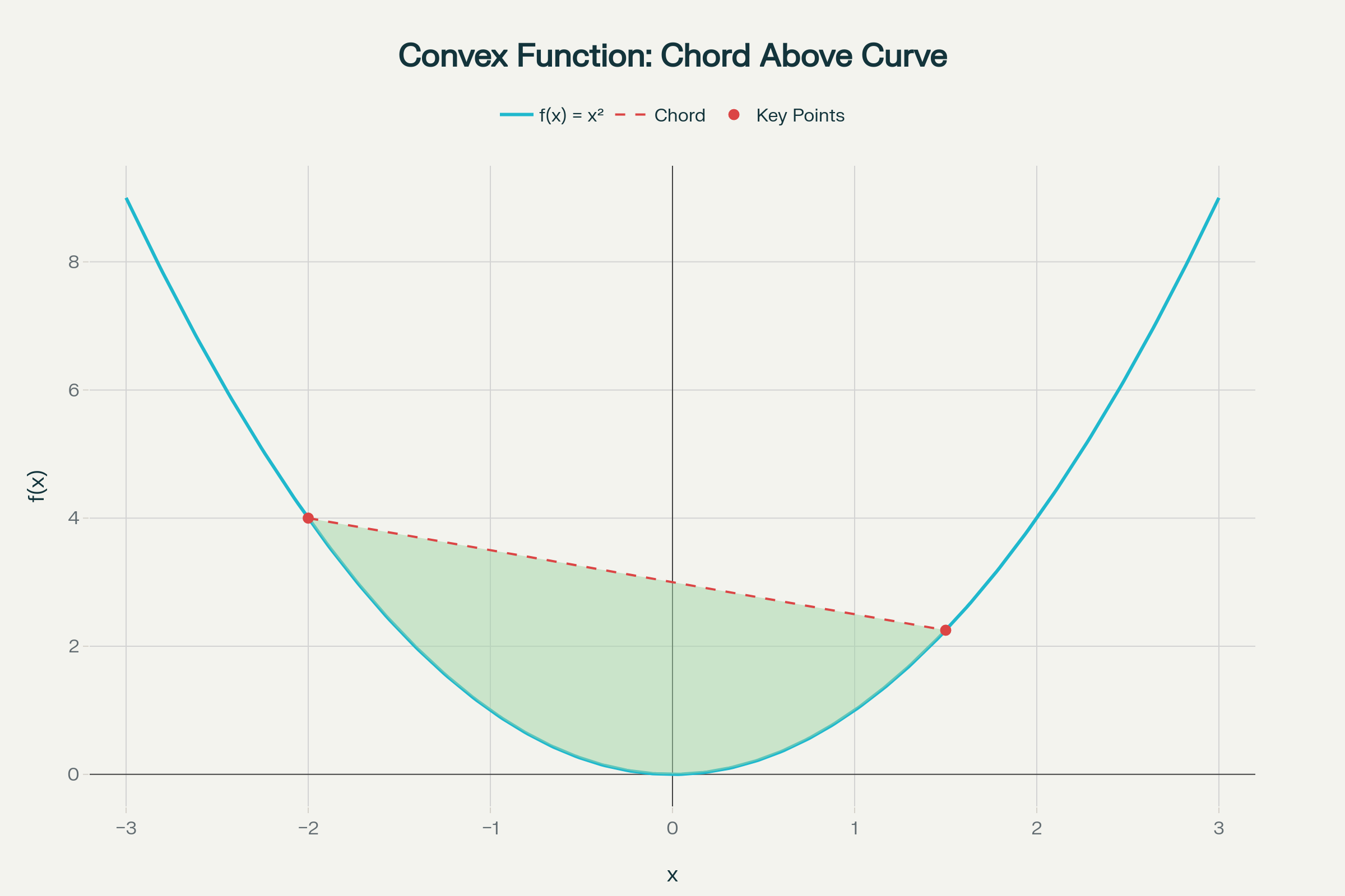
Figure 3: Convex function f. The chord (red segment) connecting two points always stays above or on the curve of f.

💡 Examples of Convex Functions

• Linear functions: \(f(x) = a^Tx + b\)
• Affine functions: \(f(x) = Ax + b\)
• Exponential: \(e^{ax}\) for any \(a \in \mathbb{R}\)
• Powers: \(x^a\) on \(\mathbb{R}_{++}\) for \(a \geq 1\) or \(a \leq 0\)
• Quadratic: \(\frac{1}{2}x^TQx + b^Tx + c\) where \(Q \succeq 0\)
• Norms: \(\|x\|_p\) for \(p \geq 1\)
• Maximum: \(f(x) = \max\{x_1, ..., x_n\}\)

📊 In dimension n

A set \(C \subseteq \mathbb{R}^n\) is convex if for all points \(x, y \in C\) and all \(\lambda \in [0,1]\), we have:

The definition remains identical—only the number of coordinates changes!

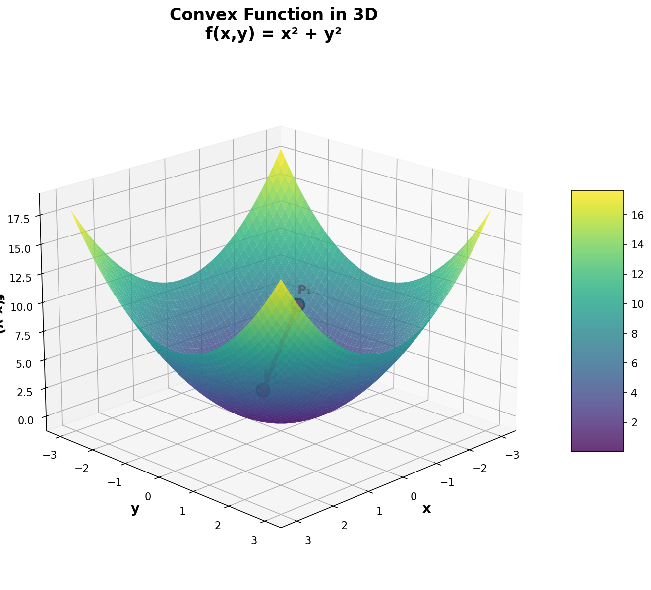
Figure 5: Convex function f(x,y) = x² + y² visualized in 3D

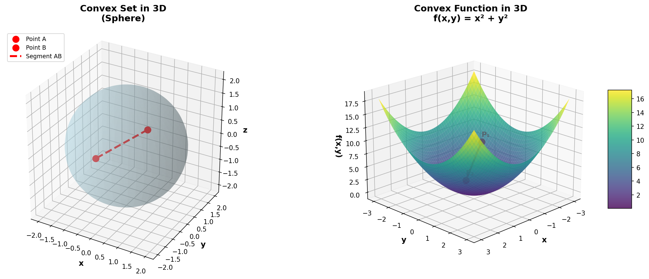
Figure 6: Left: 3D convex set (sphere) where the segment connecting two points remains in the set. Right: Convex function f(x,y) = x² + y² showing the chord above the surface.

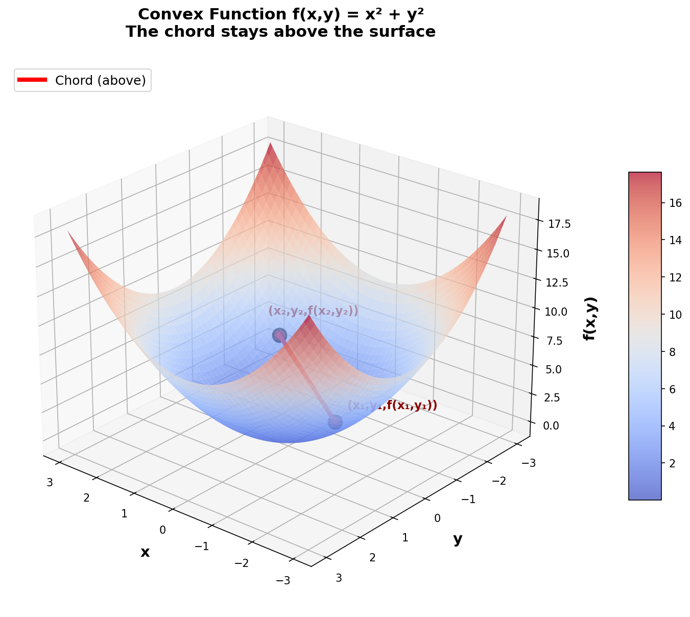
Figure 7: Detailed visualization of f(x,y) = x² + y². Green dashed lines show the vertical distance between the chord (red) and the surface, illustrating that the chord always stays above.

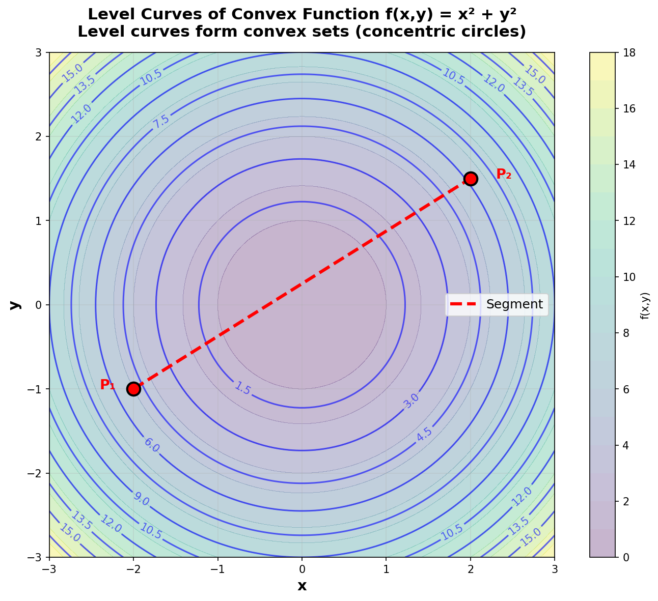
Figure 8: Level curves of f(x,y) = x² + y². The level curves of a convex function form convex sets (here, concentric circles).

🚀 Applications in High Dimensions

In practice, optimization problems often involve functions of hundreds, thousands, or even millions of variables:

• Machine Learning: Neural networks have millions of parameters
• Portfolio Optimization: Allocation across hundreds of assets
• Image Processing: Each pixel is a variable (millions of variables)
• Network Planning: Flow optimization on complex graphs

Even though we cannot visualize high-dimensional spaces, the mathematical properties of convexity (notably the uniqueness of the global minimum) remain valid and guarantee that optimization algorithms will converge to the optimal solution.

📘 Definition

For a function of several variables \(f(x_1, x_2, ..., x_n)\), the partial derivative with respect to a variable measures how the function changes when we vary that variable while keeping all other variables fixed.

Alternative notation: \(\partial_i f\) or \(f_{x_i}\)

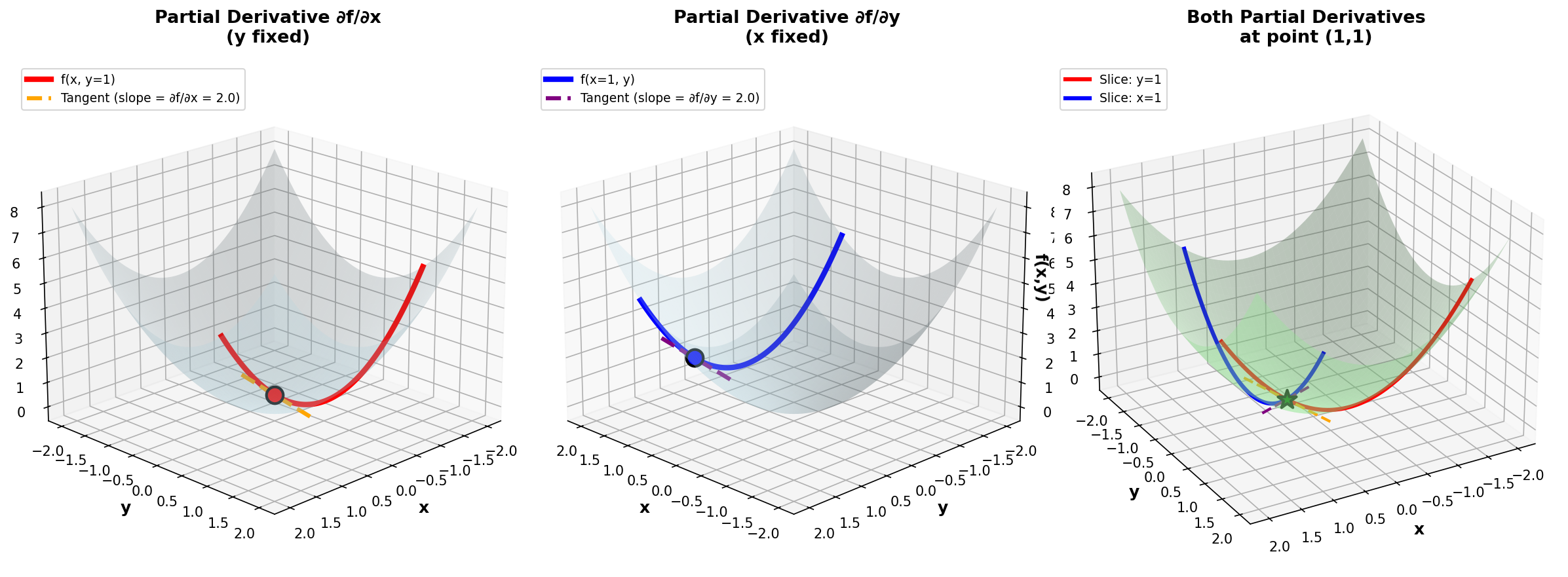
Figure 9: Partial derivatives of f(x,y) = x² + y². Left: ∂f/∂x (variation in x with y fixed). Center: ∂f/∂y (variation in y with x fixed). Right: Both partial derivatives together.

💡 Example: f(x,y) = x² + y²

Let's compute the partial derivatives:

• \(\frac{\partial f}{\partial x} = 2x\) (treating y as a constant)
• \(\frac{\partial f}{\partial y} = 2y\) (treating x as a constant)

At point (1, 2):

• \(\frac{\partial f}{\partial x}(1,2) = 2(1) = 2\)
• \(\frac{\partial f}{\partial y}(1,2) = 2(2) = 4\)

📘 Definition

The gradient is a mathematical concept used to describe the direction and rate of fastest increase of a function.

Notation: \(\nabla f\) is read as "nabla f" or "gradient of f"

🎯 Geometric Interpretation of the Gradient

• The gradient points in the direction of steepest ascent of the function (where the function increases most rapidly).
• Its magnitude \(\|\nabla f\|\) indicates the rate of this increase
• The gradient is perpendicular to level curves (or level surfaces)
• To minimize, we move in the opposite direction to the gradient: \(-\nabla f\)

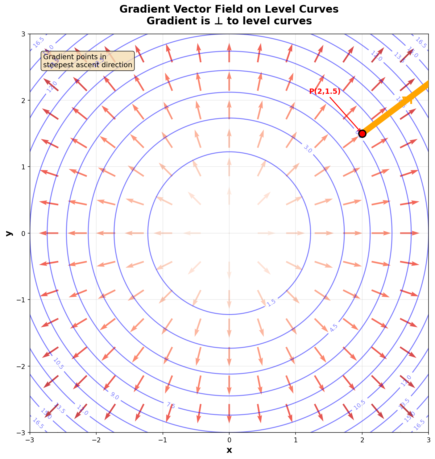
Figure 11: Gradient vector field on level curves of f(x,y) = x² + y². Arrows point outward (upward direction) and are perpendicular to circles (level curves).

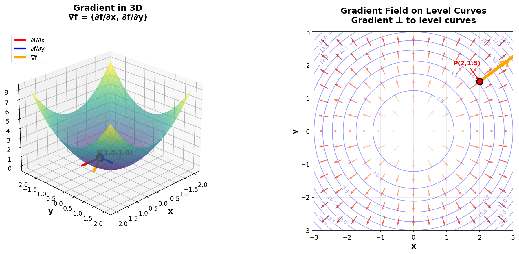
Figure 12: Left: Gradient in 3D showing how ∇f is the composition of partial derivatives (red and blue vectors give the orange vector). Right: Gradient field on level curves perpendicular to contours.

💡 Example: Gradient of f(x,y) = x² + y²

At point (3, 4):

This vector points in direction (6, 8) which is the direction of steepest ascent. Its magnitude is \(\|\nabla f(3,4)\| = \sqrt{36 + 64} = 10\), indicating the rate of growth in that direction.

📘 The Constrained Optimization Problem

We want to:

where \(f : \mathbb{R}^n \to \mathbb{R}\) is the objective function and \(g : \mathbb{R}^n \to \mathbb{R}^m\) represents the constraints.

💡 The Key Idea of Lagrange Multipliers

At the optimal point \(\mathbf{x}^*\), the gradient of the objective function \(\nabla f(\mathbf{x}^*)\) must be parallel to the gradient of the constraint \(\nabla g(\mathbf{x}^*)\).

where \(\lambda \in \mathbb{R}\) is the Lagrange multiplier.

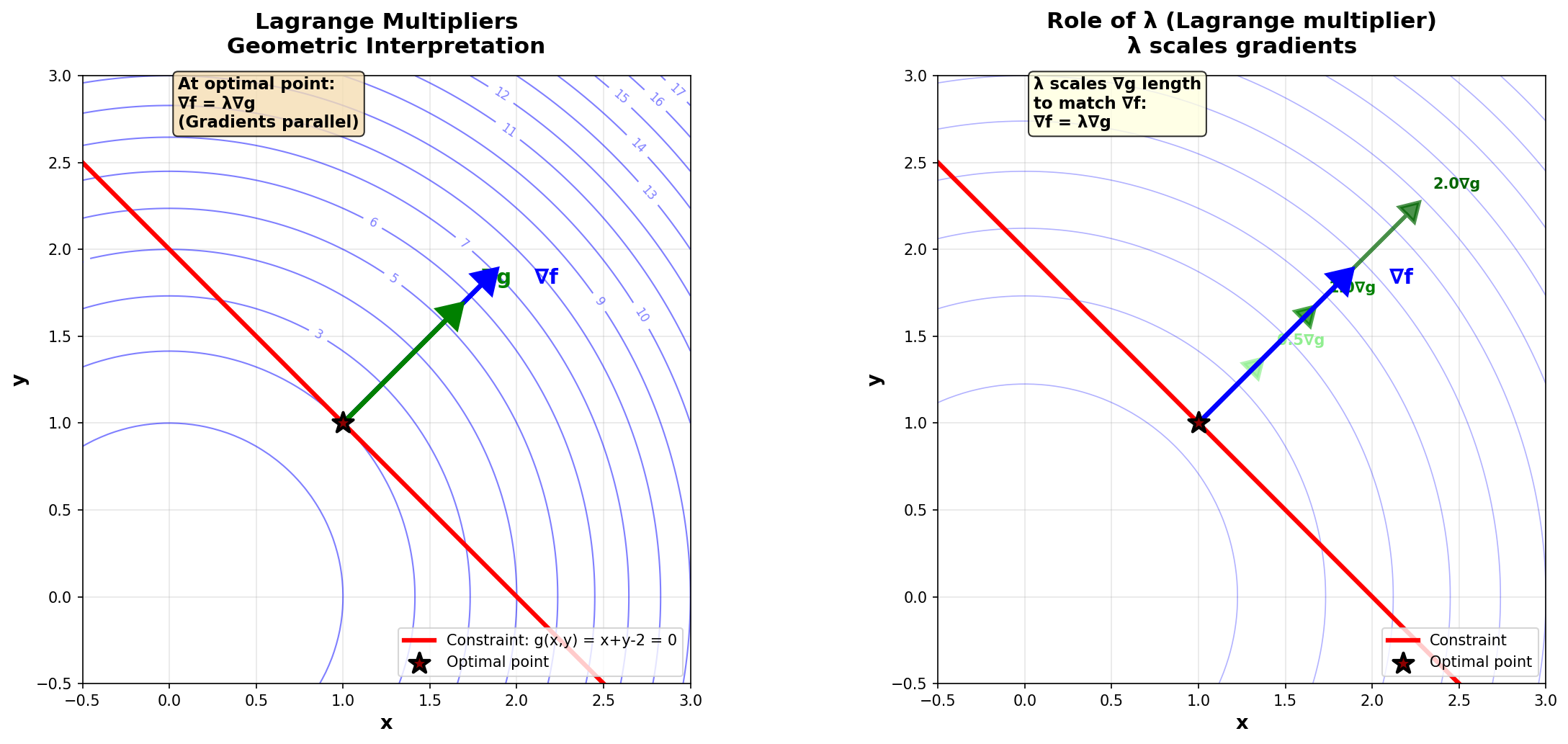
Figure 13: Geometric interpretation of Lagrange multipliers. Left: At the optimal point, ∇f (blue) and ∇g (green) are parallel. Right: The multiplier λ adjusts the length of ∇g to equal ∇f.

📘 The Lagrangian

We define the Lagrange function (or Lagrangian):

The necessary optimality conditions (Karush-Kuhn-Tucker conditions for equality constraints) are:

💡 Complete Example: Minimize f(x,y) = x² + y² subject to x + y = 2

🔍 Economic Interpretation of λ

The Lagrange multiplier \(\lambda^*\) represents the sensitivity of the objective function with respect to the constraint. More precisely, if we slightly relax the constraint from \(g(x) = 0\) to \(g(x) = \epsilon\), then:

In economics, \(\lambda\) is called the shadow price of the constraint.